Customer Churn
Overview
Customer churn rate is the percentage of customers that stop using a product within a given time frame. The goals of this project are to identify important features that help determine if a customer will churn and to build a model that will predict if a customer will churn. To achieve these goals, three models were trained and tested: Logistic Regression, Random Forest Classifier, and Gradient Boosting Classifier.
The features that were deemed as important across all three classifiers are “tenure”, “Contract_Two year”, “TotalCharges”, “InternetService_Fiber optic”, and “MonthlyCharges”. The model that had the best performance was the Random Forest Classifier with data that was oversampled and undersampled; this model resulted in an f1-score of 81% and accuracy of 82%.
1. Data
Click here to collapse section.
The Telco Customer Churn dataset is utilized in this project and can be found here. This dataset contains 7,043 unique records with 21 features:
-
Customer demographic features:
- customerID
- gender - ‘Male’ or ‘Female’
- SeniorCitizen - 1 if customer is 65 or older, 0 if not
- Partner - ‘Yes’ if customer has a partner, ‘No’ if not
- Dependents - ‘Yes’ if customer lives with dependents, ‘No’ if not
-
Service options features:
- PhoneService - ‘Yes’ if a customer signed up for home phone service, ‘No’ if not
- MultipleLines - ‘Yes’ if a customer subscribed to multiple telephone lines, ‘No’ if not, ‘No phone service’ if not applicable
- InternetService - ‘DSL’, ‘Fiber optic’, ‘No’ if customer did not subscribe to internet service
- OnlineSecurity - ‘Yes’ if a customer subscribed for this option, ‘No’ if not, ‘No internet service’ if not applicable
- OnlineBackup - ‘Yes’ if a customer subscribed for this option, ‘No’ if not, ‘No internet service’ if not applicable
- DeviceProtection - ‘Yes’ if a customer subscribed for this option, ‘No’ if not, ‘No internet service’ if not applicable
- TechSupport - ‘Yes’ if a customer subscribed for this option, ‘No’ if not, ‘No internet service’ if not applicable
- StreamingTV - ‘Yes’ if a customer uses the internet service to stream TV, ‘No’ if not, ‘No internet service’ if not applicable
- StreamingMovies - ‘Yes’ if a customer uses the internet service to stream movies, ‘No’ if not, ‘No internet service’ if not applicable
-
Customer account features:
- tenure - integer, the number of months the customer has been with the company
- Contract - ‘Month-to-month’, ‘One year’, ‘Two year’
- PaperlessBilling - ‘Yes’ if the customer enrolled in paperless billing, ‘No’ if not
- PaymentMethod - ‘Electronic check’, ‘Mailed check’, ‘Bank transfer’, ‘Credit card’
- MonthlyCharges - float, current total monthly charge for all services
- TotalCharges - float, current total charges calculated at the end of the quarter
-
Target Variable:
- Churn - ‘Yes’ if customer left the company this quarter, ‘No’ if not
2. EDA
Click here to collapse section.
Data Types
Checking the data types tells us that the TotalCharges feature is of the object data type instead of float64. The code below revealed that there are 11 blanks in TotalCharges; these blanks are converted to NaN.
# check what is causing the object data type
print([x for x in df['TotalCharges'] if any(char.isdigit() for char in x) == False])
# replace blanks with NaN
df['TotalCharges'] = df['TotalCharges'].replace(' ', np.nan)
df['TotalCharges'] = df['TotalCharges'].astype('float64')
Target Variable
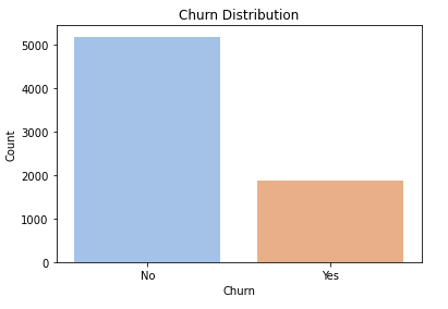
There is an imbalance in the target variable that will be addressed after taking a look at the features in the dataset:
- Customers that did not churn: 5174 or approximately 73%
- Customers that did churn: 1869 or approximately 27%
Numerical Features
We will examine the numerical features first. Below we have the relationship between churn rate and tenure. The churn rate is calculated by dividing the number of churns by the total number of customers for each unique value of tenure.
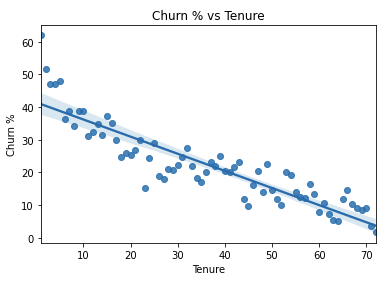
We see that there is a negative correlation between churn rate and tenure. This suggests that the longer a customer has been with the company, the less likely the customer will churn. For MonthlyCharges and TotalCharges, we can compare the distributions using layered histograms.
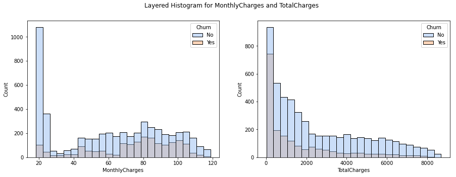
We can see in MonthlyCharges that there is a sharp peak for customers that do not churn at the $20 range, otherwise the distributions for Churn = ‘Yes’ and Churn = ‘No’ follow a similar pattern for this feature. The distributions for TotalCharges are both skewed right.
Now that we have analyzed the numerical features, we can fill in missing values for TotalCharges:
df['TotalCharges'].fillna(df['TotalCharges'].mean(), inplace=True)
Categorical Features
Demographics
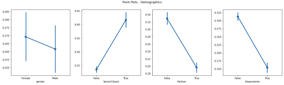
Next we can take a look at the point plots and churn rate breakdown for demographic features:
| gender | No | Yes | Churn % |
|---|---|---|---|
| Female | 2544 | 939 | 26.96 |
| Male | 2619 | 930 | 26.20 |
| SeniorCitizen | No | Yes | Churn % |
|---|---|---|---|
| False | 4497 | 1393 | 23.65 |
| True | 666 | 476 | 41.68 |
| Partner | No | Yes | Churn % |
|---|---|---|---|
| False | 2439 | 1200 | 32.98 |
| True | 2724 | 669 | 19.72 |
| Dependents | No | Yes | Churn % |
|---|---|---|---|
| False | 3390 | 1543 | 31.28 |
| True | 1773 | 326 | 15.53 |
- gender: appears to be the only demographic feature where the churn rate for each class are not so different
- SeniorCitizen: customers who are 65 or older are approximately 2.3 times more likely to churn than customers who are not
- Partner: customers who do not have a partner are approximately 2 times more likely to churn than customers who do have partners
- Dependents: customers that do not have dependents are 2.4 times more likely to churn than customers who live with dependents
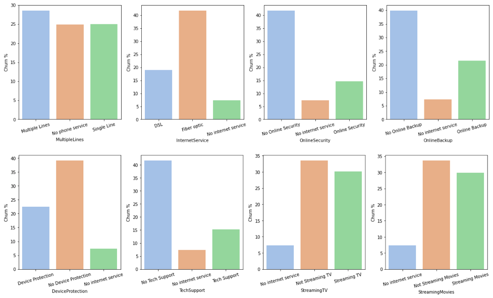
Service Options
Below we have the churn rates for the values in the service options features. We can see that the churn rate varies for the categories within the features. For instance, the ‘Fiber optic’ option in InternetService has a churn rate that is at least 10% higher than the other values for this feature.
We can also look at the relationship between various features by creating a stratified contingency table. Here are a couple of examples:
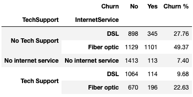
First we have the stratified contingency table of TechSupport and InternetService. Customers that have ‘No Tech Support’ and the ‘Fiber optic’ option of InternetService have a churn rate of 49.37%. That is pretty high and it may be worth the company looking into. On the other hand, customers that have ‘Tech Support’ and the ‘DSL’ option of InternetService have a churn rate of 9.86%. Why is there a low churn rate for this combination of features? Can something be learned from this and applied to customers that have ‘Fiber optic’ with ‘No Tech Support’?
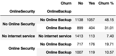
Next we have the stratified contingency table of OnlineSecurity and OnlineBackup. Here we see a stark difference between customers who have ‘No Online Security’ and ‘No Online Backup’ and customers who have ‘Online Security’ and ‘Online Backup’. Is there a way to encourage ‘Online Security’ and ‘Online Backup’ in order to lower the churn rate?
Customer Account
Repeating the steps made for the service options features, below we have the churn rates for the values in the customer account features.
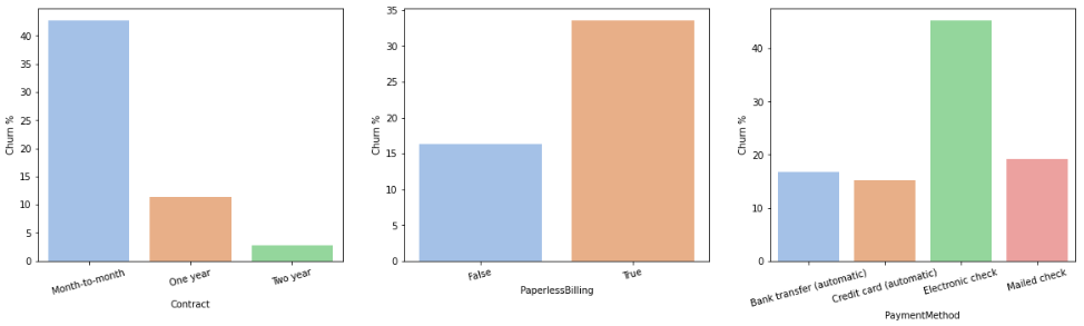
Again, we can see that the curn rate varies for the categories within the features. For instance, the ‘Electronic check’ option in PaymentMethod has a churn rate that is at least 25% higher than the other values in PaymentMethod and the ‘Month-to-month’ option in Contract has a churn rate that is at least 30% higher that the other values in Contract. Let’s look at a couple of stratified contingency tables for this set of variables:
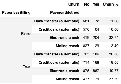
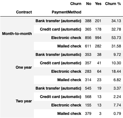
First we have the table for PaperlessBilling and PaymentMethod. We can see that there is an overall pattern of paperless billing leading to higher churn rates. Below we have the table for Contract and PaymentMethod. ‘Month-to-month’ contracts paid with ‘Electronic check’ have a high churn rate of almost 54% while the same contract paid with a ‘Mailed check’ has a significantly lower churn rate of 31.58%.
Dealing with Imbalanced Target Variable
Now we can address the imbalanced target variable. In this dataset there are 5,174 customers that did not churn and 1,869 customers that did churn. We will take two steps to try to overcome the imbalance:
- Use f1-score to measure the accuracy of the models
- Combine random oversampling and random undersampling
from imblearn.over_sampling import RandomOverSampler
from imblearn.under_sampling import RandomUnderSampler

X_df = df.drop('Churn', axis=1).copy()
y_df = df['Churn'].values

ros = RandomOverSampler(sampling_strategy=0.6)
X_ros, y_ros = ros.fit_resample(X_df, y_df)

rus = RandomUnderSampler(sampling_strategy=0.8)
X_co, y_co = rus.fit_resample(X_ros, y_ros)

sampling_df = X_co.copy()
sampling_df['Churn'] = y_co
This resulted in a new dataset that consists of 6,984 records with 3,880 customers that did not churn and 3,104 customers that did churn. Information on the f1-score can be found here. A tutorial for random oversampling and undersampling can be found here.
3. Data Cleaning
Click here to collapse section.
Now that we have an overview of the variables in the dataset and have modified the dataset to overcome the imbalanced target feature, we can encode our data. First we split the dataset into X (independent variables) and y (target variable), then we can encode all of the categorical features. We have seven categorical features that are binary and will be encoded using label encoding: Churn (our y), gender, SeniorCitizen, Partner, Dependents, PhoneService, and PaperlessBilling. The remaining categorical features will be encoded using one-hot-encoding: MultipleLines, InternetService, OnlineSecurity, OnlineBackup, DeviceProtection, TechSupport, StreamingTV, StreamingMovies, Contract, and PaymentMethod:
from sklearn import preprocessing

X_df = sampling_df.iloc[:, 1:-1].copy()
y = sampling_df.iloc[:, -1].values

# encoding binary categorical variables:
binary_col = ['gender', 'SeniorCitizen', 'Partner', 'Dependents',
              'PhoneService', 'PaperlessBilling']

for col in binary_col:
    le = preprocessing.LabelEncoder()
    X_df[col] = le.fit_transform(X_df[col])

# one-hot-encoding for the remaining categorical variables:
remaining_col = ['MultipleLines', 'InternetService', 'OnlineSecurity', 'OnlineBackup', 'DeviceProtection',
                 'TechSupport', 'StreamingTV', 'StreamingMovies', 'Contract', 'PaymentMethod']

X_df = pd.get_dummies(X_df, columns=remaining_col, drop_first=True)
X = X_df.values

# class encoding:
le_class = preprocessing.LabelEncoder()
y = le_class.fit_transform(y)
We then split the dataset into training and testing sets using the train_test_split function from scikit-learn and scale the features as well:
from sklearn.model_selection import train_test_split

# 60/40 train/test split:
X_train, X_test, y_train, y_test = train_test_split(X, y, test_size=0.4, random_state=1)

# 20/20 test/validation split:
X_test, X_val, y_test, y_val = train_test_split(X_test, y_test, test_size=0.5, random_state=1)

# scale features
stdsc = preprocessing.StandardScaler()
X_train_std = stdsc.fit_transform(X_train)
X_test_std = stdsc.transform(X_test)
X_val_std = stdsc.transform(X_val)

# we want to preserve the column names for later
X_train_std = pd.DataFrame(X_train_std)
X_train_std.columns = X_df.columns
4. Model Building with Scikit-Learn
Click here to collapse section.
We are ready to build our models. For this project, we will train Logistic Regression, Random Forest, and Gradient Boosting classifiers and find the optimal hyperparameters for each model using GridSearchCV.
Logistic Regression
First we will build the Logistic Regression model. Using GridSearchCV, we can try different values for the hyperparameter ‘C’ and check which value gives us the highest f1 score.
from sklearn.linear_model import LogisticRegression
from sklearn.model_selection import GridSearchCV

lr = LogisticRegression(random_state=1)

parameters = {
    'C': [0.001, 0.01, 0.1, 1, 10, 100, 1000]
}

lr_cv = GridSearchCV(estimator=lr, param_grid=parameters, scoring='f1', cv=5)
lr_cv.fit(X_train_std, y_train.values.ravel())
print('Mean Test Scores:', lr_cv.cv_results_['mean_test_score'])
The average f1 results for each value of ‘C’ are: 74.8%, 75.2%, 75.6%, 75.5%, 75.6%, 75.7%, and 75.7%. Since C=100 has the highest f1 score, this is the hyperparameter that will be used in the Logistic Regression model.
Random Forest
Next we will build the Random Forest classifier. Here, we will try different values for three hyperparameters (n_estimators, max_features, and max_depth) and find which combination of these values will result in the highest f1 score.
from sklearn.ensemble import RandomForestClassifier

rf = RandomForestClassifier(random_state=1)

parameters = {
    'n_estimators': [5, 25, 50, 100, 250],
    'max_features': ['auto', 'sqrt', 'log2'],
    'max_depth': [2, 4, 8, 16, 32, 64, None]
}

rf_cv = GridSearchCV(estimator=rf, param_grid=parameters, scoring='f1', cv=5)
rf_cv.fit(X_train_std, y_train.values.ravel())
print('Mean Test Scores:', rf_cv.cv_results_['mean_test_score'])
The combination of values that resulted in the highest f1 score of 79.7% are max_depth = 16, max_features = log2, and n_estimators = 100. This combination will be used for the hyperparameters of the Random Forest classifier.
Gradient Boosting
Lastly, we will build the Gradient Boosting classifier. The hyperparameters that will be tuned for this model are n_estimators, max_depth, and learning_rate.
from sklearn.ensemble import GradientBoostingClassifier

gb = GradientBoostingClassifier(random_state=1)

parameters = {
    'n_estimators' : [5, 50, 100, 250, 500],
    'max_depth' : [2, 4, 6, 8, 10],
    'learning_rate' : [0.01, 0.1, 1, 10, 100]
}

gb_cv = GridSearchCV(estimator=gb, param_grid=parameters, scoring='f1', cv=5)
gb_cv.fit(X_train_std, y_train.values.ravel())
print('Mean Test Scores:', gb_cv.cv_results_['mean_test_score'])
The combination of values that resulted in the highest f1 score of 78.2% are n_estimators = 500, max_depth = 8, and learning_rate = 0.01. This combination will be used for the hyperparameters of the Gradient Boosting model.
5. Feature Selection
Click here to collapse section.
To find what features are the most relevant for determining customer churn, we can utilize SelectFromModel from scikit-learn. This transformer allows us to select features based on importance weights. After running SelectFromModel on each model, these are the features that were selected:
| Model | Selected Features |
|---|---|
| Logistic Regression | tenure, MonthlyCharges, TotalCharges, InternetService_Fiber optic, StreamingMovies_Streaming Movies, Contract_Two year |
| Random Forest | tenure, MonthlyCharges, TotalCharges, InternetService_Fiber optic, Contract_One year, Contract_Two year, PaymentMethod_Electronic check |
| Gradient Boosting | tenure, MonthlyCharges, TotalCharges, InternetService_Fiber optic, Contract_One year, Contract_Two year |
Features that were chosen across all classifiers: tenure, Contract_Two year, TotalCharges, InternetService_Fiber optic, and MonthlyCharges.
Features that did not appear in any of the chosen optimal models: gender, SeniorCitizen, Partner, Dependents, PhoneService, PaperlessBilling, MultipleLines_No phone service, MultipleLines_Single Line, InternetService_No internet service, OnlineSecurity_No internet service, OnlineSecurity_Online Security, OnlineBackup_No internet service, OnlineBackup_Online Backup, DeviceProtection_No Device Protection, DeviceProtection_No internet service, TechSupport_No internet service, TechSupport_Tech Support, StreamingTV_Not Streaming TV, StreamingTV_Streaming TV, StreamingMovies_Not Streaming Movies, PaymentMethod_Credit card (automatic), and PaymentMethod_Mailed check.
It is worth noting that the features that were chosen/not chosen may change depending on the records selected in the oversampling/undersampling step.
6. Model Selection
Click here to collapse section.
Now that we have built and tuned our models, we can test the models on the validation set and choose the model that performs the best. The resulting accuracy and f1 scores are as follows:
| Model | Accuracy | F1 Score |
|---|---|---|
| Logistic Regression | 74.52 | 72.45 |
| Random Forest | 80.82 | 78.90 |
| Gradient Boosting | 79.17 | 77.56 |
The Random Forest classifier performed the best with the highest accuracy and f1 score. We will use the Random Forest model on the test set and plot the confusion matrix.
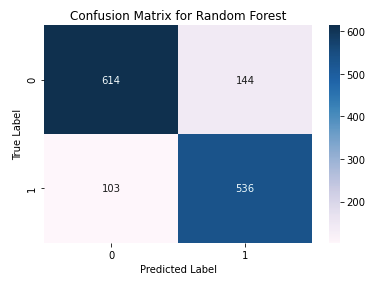
The accuracy on the test set is 82.32% and the f1 score is 81.27%. In the confusion matrix above, we see that that the true label ‘1’, or ‘Yes’, was incorrectly predicted as ‘0’, or ‘No’, 103 times. We also see that the true label ‘0’ was incorrectly predicted as ‘1’ 144 times.
Overall, Random Forest Classifier with data that was oversampled and undersampled performed the best with an f1-score of 81% and accuracy of 82%.